Pythagorean Roulette

Last time we derived the gravity-based equation that powers interstellar travel in gr_4Xity. The “jump distance” to another star is determined by a square root function that captures diminishing returns.

Square-root distance functions arise in many different contexts. In this article, we’ll apply another example that’s critical to crafting variation and risk in the world and gameplay of gr_4Xity. In building tools to carefully manage the design and implementation of randomness, we embrace Chaoskampf Studios’ titular struggle against chaos. We’ll go further than popular game engines to develop functionality more typical of the numerical computing platforms used by statisticians, data scientists, and machine learning engineers.

A Uniform Start

While not all games incorporate chance, traditional board, arcade, and casino games that do so use some physical mechanism–tossing coins, rolling dice, shuffling cards, spinning a wheel, pulling a plunger, etc. True mechanical randomness isn’t feasible from a digital computer, but software development platforms almost always include a core feature for “pseudo”-random numbers good enough for practical use (including modern digital casino games). This is true of popular game engines as well:

Roblox’s NextNumber “Returns a pseudorandom number uniformly distributed over [0, 1).”
Godot’s randf “Returns a pseudo-random float between 0.0 and 1.0 (inclusive).”
Unity’s Random.value “Returns a random float within [0.0..1.0]”
Unreal’s Random Float “Returns a random float between 0 and 1”

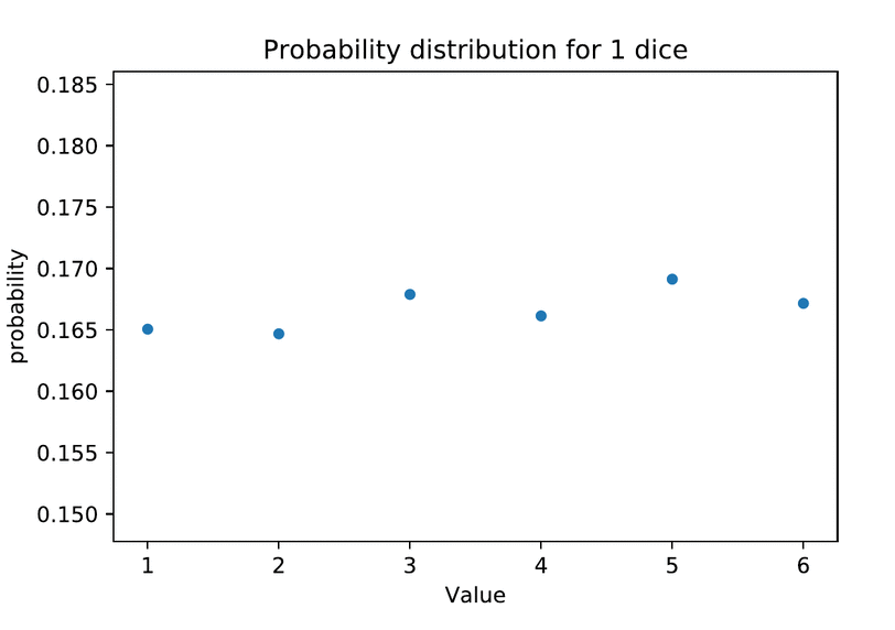
Details, implementations, and quality of documentation vary, but this core pseudo-random functionality always starts with some uniform distribution where each outcome is equally likely–ala each side of a fair coin or die. Computers can conjure up digital dice of any number of sides, effecting a continuous uniform distribution as the number of sides reaches the limit of their numerical precision.

Between 0 and 1 is the “standard” for a continuous uniform distribution. This is handy because probability is bounded between 0% and 100%, allowing direct application of simple probabilistic rules. For example, if the probability of a spearman defeating a tank is 1%, the game logic can be easily expressed:

C-style


if standard_uniform() < 0.01 {
    spearman_wins()
} else {
    tank_wins()
}

Rebol-style

case [
    standard-uniform < 1% [
        spearman-wins
    ]
    else [tank-wins]
]

Note that we’ll typically use the more friendly Rebol (or Ren) syntax for (pseudo)code instead of the archaic C-style, which requires heavy use of the shift operator to underscore word separation, parenthesize function arguments, and control flow with curly brackets [“C” must be short for Carpal Tunnel Syndrome!].

Many chance-based mechanics in video games are constructed with such probability-based rules, directly in code or data-driven with lookup tables. And from this simple tool, it’s easy to see how more flexible uniform random number generators can be constructed to go beyond the standard range with additional operations. For example:

Translation: Adding or subtracting a number shifts the position of the distribution up or down, while preserving the absolute distance between each unit. For example, 0.75 and 0.25 are 0.50 units apart, and if we add 2 to both numbers they’re still 0.5 units apart [2.75 – 2.25 = 0.50].
Scaling: Multiplying or dividing by a number changes the scale of the distribution to make it wider or narrower, while preserving the relative distance between each unit. For example, 0.75 is 3 times as large as 0.25, and if we multiply both numbers by 2 the first is still 3 times as large [1.5 / 0.5 = 3].
Discretization: Truncating and rounding allow continuous distributions to produce discrete outcomes.

Some game engines provide higher-level functions to combine these operations under a simpler interface, allowing game designers and programmers to spec and implement chance events directly in characteristic terms rather than via the chain of mathematical operations needed to get there. Any uniform distribution can be characterized with just two numerical parameters–by convention typically the minimum and maximum value over its range. For example:

Roblox’s NextInteger “Returns a pseudorandom integer uniformly distributed over [min, max].”
Godot’s randi_range “Returns a pseudo-random 32-bit signed integer between from and to (inclusive).”
Unreal’s Random Integer in Range “Return a random integer between Min and Max (>= Min and <= Max)”
Unity like many others requires you to roll your own!

These high-level functions make it easy to model coin, dice, and card mechanics in video games. But uniform distributions don’t directly address all chance-based operations. What about game systems that don’t reduce to simple probability rules or where not all outcomes are equally likely?

Normal Means

In 1809, Carl Friedrich Gauss published Theory of the Motion of the Heavenly Bodies Moving about the Sun in Conic Sections. One of the achievements he detailed was his Gaussian gravitational constant–equivalent to the square-root of G in Newton’s gravity equation that we used in the prior entry.

But it’s Gauss’s development of modern statistics in the same text that concerns us here. He described the “normal” or “Gaussian” distribution to characterize measurement errors in astronomy. Typically errors were small, clustered in the center, but there were diminishing tails of rare under- and over-measurement on either side.

https://wumbo.net/concepts/normal-distribution/

This pattern–most outcomes around the middle (a central tendency) with symmetric variation on either side–occurs often in science and nature, as well in our measurements of such phenomena. Like the uniform distribution, it can be characterized by just two numbers. In this case, we want to know (or estimate) the location of the central tendency (population mean µ), as well as how wide-spread or dispersed it is on average around this center (standard deviation σ):

This “standard deviation” is another square-root based distance formula, but not the ultimate goal of this article. It’s useful to measure the dispersion of a normal distribution in the same units as the mean and the data itself. But we often talk about it’s square, the variance (σ²), which is easier to estimate without bias.

What Gauss had to say about the arithmetic mean (µ) is more interesting. Taking an arithmetic average is equivalent to linear regression. Gauss developed the method of least squares., which provides a powerful interpretation of the average as a measure “closest” to any set of data–the point that minimizes total variance.

Consider the residual distance between each observation y_i and some point µ. Distance is squared in the physical gravity equation because of the bidirectional force of attraction; here we’ll square distance so positive and negative values don’t wash out–to penalize variance. For example +1 and -1 are closer together than +2 and -2, so while both pairs are centered around zero the latter is “noisier”. We’ll add-up these squared distances to get a total measure of deviation, typically called the “Residual Sum of Squares” (RSS):

You’ll note this is the inner core of the definition of the standard deviation, prior to averaging over all n and taking the square root. Here it’s the total rather than the average deviation we care about, and taking the square root complicates the math without affecting the solution to the following problem.

Our goal is to choose µ in order to minimize this total squared error. The minimum occurs at the bottom of the valley where the slope is flat, so to find it we set the derivative equal to zero:

A bit more algebra to solve for µ yields the RSS-minimizing solution, which is simply the arithmetic mean:

This variance-minimizing property of the simple average is true for any data of any distribution. Whether that mean is meaningful or actionable are separate questions.

Gauss went there, asking what shape data must be in for the average to capture some fundamental character of the data. His answer was this symmetrically bell-shaped “Gaussian” curve. In Gauss’s definition, data is “normal” if the arithmetic mean does more than just minimize the total of squared deviations–it also estimates the most-likely location of the central tendency, the median.

In contrast, the uniform distribution has no central tendency. The average of a uniform distribution is indeed closest to all outcomes, but it’s no more or less likely than any other result. If you’re facing an individual draw from the uniform distribution, the mean may be meaningless.

It’ll be useful here to start making a distinction between population statistics which capture the entirety of a problem space and sample statistics which are derived from a subset the population. Rarely are we omniscient; most often we need to draw inferences about a population from samples that may or may not be representative. The sampling process itself becomes the process of interest.

Monte Carlo, New Mexico

The characteristic shape of the normal distribution is the result of an additive data generating process. We can achieve it simply by adding up a number of independent samples from the same uniform distribution, for example by accumulating repeated dice rolls.

Thanks to Tom Leyshon: “Modelling the probability distributions of dice” on TDS.

This “Monte Carlo method” of simulating repeated random sampling to generate distributions was inspired by card games–specifically Solitaire–but the name itself was a military code. The method comes to us from this author’s hometown of Los Alamos, New Mexico, developed by Stanisław Ulam along with his work on the Manhattan Project.

Consider another example, tabletop role-playing games like Dungeons & Dragons (and their digital inspirations). Making contact with an enemy is typically a matter of probability handled with a uniform distribution, rolling independent 20-sided “hit dice” for each attack (a d20 breaks continuous probability into discrete 5% chunks). Then, damage is often dealt pseudo-normally, rolling and adding up multiple smaller dice from one or more successful hits–especially at higher levels. Various effects apply translations to both distributions. The core player action loop of independent uniform rolls to hit then cumulative rolls for pseudo-normal damage determines the flow and balance of combat encounters in these experiences as well as the trade-offs players make in character progression.

The intuition to how normality emerges here is simple. When we average multiple independent draws from the same uniform distribution, on average higher and lower numbers cancel each other out, with some regularly expected variation to the degree they don’t. If we roll two 6-sided dice, there’s only one way to total a 2 or 12 at the tails, but a half-dozen different outcomes sum to the most likely middle-ground at 7. Dividing in half yields 3.5–the same arithmetic mean as one roll or an infinite number of rolls–so averaging simply rescales the total area under the curve of the sample distribution onto the same scale as the individual samples. But the more dice we roll, the narrower the variance around the mean.

It takes a little more math to standardize the resulting accumulation, providing a high-level interface to implement a standard normal distribution centered at zero with a standard deviation of one. Applying our knowledge the standard uniform distribution to translate and scale cumulative results is straight-forward: demean by subtracting the average contribution from the standard uniform’s mean (1 / 2) for each n samples, then deflate by a square-root distance function to correct for noise that decreases at a diminishing rate with the number of samples relative to the standard uniform’s variance (1 / 12).

A simple function that takes the number of samples as an optional parameter might look something like this (comments followed by a semi-colon):

mc-standard-normal: function [
    {Returns a pseudorandom float! from the standard normal 
     distribution, approximated by Monte Carlo simulation}
    /samples n [integer!] "Number of independent uniform samples"
][
    unless n [n: 1000]  ; default to some large sample size
    s: 0.0              ; initialize sum
    loop n [s: s + standard-uniform]  ; accumulate each sample
    return (s - (n / 2)) / (square-root (n / 12)) ; standardize
]

This provides a basis for higher-level functions with user-specified characteristic mean and standard deviation (or variance) as parameters.

Generating a normal distribution in this fashion is an application of the Central Limit Theorem. With a large enough number of trials, rough normality emerges from repeatedly sampling a source distribution of any shape. When we attempt to estimate the arithmetic mean of a population using a sample of data, the sampling process itself introduces noise into our summing and averaging. Most of the time the resulting sample mean should be close to the population mean–however it’s determined–with decreasing likelihood of larger errors on either side. Gauss’s bell curve arises directly from the measurement process of computing and comparing arithmetic means from related samples–hence why Gauss himself found this shape in charting measurement errors.

This makes the Central Limit Theorem a powerful tool, though an often over-interpreted one. Normality only emerges from the additive process of summing sample observations, so it only applies to the arithmetic sum and average–not to other population parameters–like the minimum and maximum characteristic of a uniform distribution. While linear regression via least squares may “work” in many circumstances to estimate the population mean of any distribution, Gauss’s insight still applies: this only estimates the central tendency (the median) of an effect when the effect itself is normally distributed in the population. When we rely on the Central Limit Theorem to estimate some arithmetic mean of a non-normal process, hypothesis testing based on the estimated deviation from the sample mean only addresses how reliable our measurement of the average is given sampling error–not the reliability of the effect itself in the population.

This often leads to insufficient identification and control in experiments, which in turn leads to failed replicability. For example, suppose the arithmetic mean of some uniformly-distributed process is 5% higher in a test group than a randomized control group. Is this because of a higher minimum, higher maximum, or some other combination (e.g. much higher min but somewhat lower max, or vice versa)? Understanding the underlying data-generating process and pursuing more characteristic measures can lead to more robust and actionable insights.

As Ulam realized, computers can repeat and operate on random samples much faster than us humans. Still, one might wish to avoid generating a large number of random numbers to produce a single normally-distributed random output. Is there a more direct, more efficient way to achieve the desired behavior?

Step Up and Take a Spin

While the shape of the normal distribution is clearly specified mathematically, unfortunately there’s no analytical solution to the problem of inverting this knowledge to transform a uniform distribution directly to normality. Approximations introduce significant error.

Undeterred, mathematicians George E.P. Box and Mervin E. Muller published a creative solution in 1958. Consider a simple circle:

Planetary orbits are elliptical–not perfectly circular–but forgive adding a little contextual color to the illustration!

Source [red-lang] | Windows (zipped exe) | Linux (tgz)

Given some angle (θ) and radial distance (r), we can use simple trigonometric functions to transform these parameters into spatial coordinates representing a point in 2D space:

Suppose we randomly choose the angle (θ) and radial distance (r). Can we make these random draws in a way that solves our problem?

Let’s start by assuming x and y are independent standard normal distributions. Their joint probability density is the product of their individual density functions:

Recall the Pythagorean Theorem:

such that we can define the radius of our circle by yet another square-root distance function:

Applying this to our joint probability density:

This is a constant times an exponential function. Thus the joint distribution of two independent standard normals, x and y, is equivalent to the joint distribution of a uniform distribution between 0 and 2π and a standard exponential distribution, each also independent.

Choosing a uniformly-distributed random angle between 0 and 2π radians (between 0° and 360°) is easy with the basic tools provided by any programming environment–just multiply draws from the standard uniform distribution by 2π. A roulette wheel provides a discrete, mechanical model of this process.

Let’s add another dimension to our wheel to capture distance from the center. An exponential distribution makes intuitive sense to generate outcomes that cluster close to the origin, as it models decay starting from some initial value. This constant rate of decay is already normalized to the standard λ=1, which is easier to see if we define a variable z to simplify the density function:

where

The radial distance is still a square-root function, via the Pythagorean Theorem, but now is expressed directly in terms of a sample from the standard exponential distribution!

Note that while the exponential distribution has no central tendency, it can be meaningfully characterized by the arithmetic mean; the expected average lifespan is the inverse of the rate of decay. Exponential distributions are often used to model decay in time, but duration is a valid measure of distance over time so spatial applications like this come naturally as well.

Unlike for the normal distribution, it’s possible to directly transform a uniform distribution to exponential by cumulating and inverting the probability density function (inverse transform sampling). This lets us do things like directly compute quantiles for the exponential distribution, as well as apply a non-linear transform to generate exponentially-distributed samples (z) from uniformly-distributed probability (0 <= p < 1):

Non-linear transformations like this change both absolute and relative measures of distance, moving us to a completely different scale of measurement.

All together now, we have our final square-root distance functions:

This ingenious Box-Muller transform takes two independent samples from the standard uniform distribution (p₁ and p₂) and generates two independent samples from the standard normal distribution (x and y) which can be interpreted as 2D noise around a zero center. Here’s a sample implementation in code:

box-muller: function [
    {Returns a set of two independent pseudorandom float!
     from the standard normal distribution.}
][
    theta: 2 * pi * standard-uniform
    r: square-root -2 * (ln 1 - standard-uniform)
    reduce [
        r * cos theta
        r * sin theta
    ]
]

The following visualization applies this code in a Monte Carlo simulation. Each sample is a 2D coordinate generated by the Box-Muller transform from two draws from the standard uniform distribution. These create a scatterplot (in green).

Sour ce [red-lang] | Windows (zipped exe) | Linux (tgz)

The histograms along the upper X and lower Y axes accumulate the x and y coordinates (in blue and yellow) from each successive sample, sketching out the two independent normal distributions that emerge from the repeatedly sampling.

The cross and circles (in white) plot the theoretical population mean and +1/+2/+3 standard deviations of the expected normal distributions. Commensurate sample estimates (in green) are updated with each iteration, and these converge as expected toward the population values as the number of samples increases.

Log-Normality

As we showed in the prior entry, space travel in gr_i4Xity depends on the spatial distribution of mass. In our Milky Way, red dwarfs smaller than our sun are far more common than massive giant stars. If stellar mass in gr_i4Xity was uniformly distributed–stars of any mass equally likely–it would break both gameplay and immersion. So too would the normal distribution, which would make giants symmetrically likely as dwarfs.

A “log-normal” distribution solves this problem. While additive processes generate normal distributions, multiplicative processes result in log-normality. Because gravity itself is a multiplicative process, over time it pulls the initial distribution of matter from the Big Bang into roughly log-normally distributed agglomerations: stars and planets and asteroids and comets.

Unlike in the normal distribution where the arithmetic mean estimated the location of the median, under log-normality the simple average is biased upward by the skew of the long tail to the right. Instead, an unbiased estimate of the median central tendency is given by the geometric mean (g):

Thus the log-normal distribution is characterized by the geometric mean (g) and the multiplicatively-symmetric geometric deviation (h) (or geometric variance h²) around it.

What would happen if we multiplied a set of uniform dice rolls instead of summing them? Starting with two 6-sided dice, for example, we’d see the range is much broader, from 1X1=1 to 6X6 = 36. Most outcomes would be closer to the lower limit than the extreme high. While the arithmetic mean of any number of d6 is 3.5, the geometric mean and thus population median are lower at approximately 3.

The geometric equivalent of the Central Limit Theorem says that the error in our estimate of the geometric mean from repeated independent draws from an identical distribution of any shape becomes log-normally distributed as the number of samples increases. We could apply this to generate a log-normal distribution through Monte Carlo simulation of a large numbers of samples.

Fortunately, now that we’ve solved our normal distribution generation problem, there’s a better way. Just like we were able to transform a uniform distribution into an exponential distribution with an inverse operation (the natural log), we’re able to transform a normal distribution to log-normality by exponentiation.

Note that the arithmetic mean of a log-normal distribution depends only on the characteristic geometric mean and variance. It’s the geometric variance (h²) that raises the arithmetic mean above the central geometric mean, creating a tradeoff since more individual risk comes with a higher average reward.

Chaoskampf Studios has often found it convenient in design to specify log-normal distributions in terms of the median (geometric mean) and average (arithmetic mean), using the above relationship to infer and manage geometric variance accordingly. Here’s a simplified version of the source code for the high-level log-normal generating function from gr_4Xity‘s custom game engine:

next-lognormal: func [
    {Returns a pseudorandom float! from lognormal distribution}
    gm [number!] "Median central tendency (geometric mean)"
    am [number!] "Arithmetic mean > geometric mean"
    /local norms
][
    norms: []  ; allocate once, modify each function call
    if empty? norms [
        append norms box-muller  ; cache 2 at a time
    ]
    exp (ln gm) + ((pop norms) * (square-root 2 * (ln am / gm)))
]

For example:

>> next-lognormal 3 3.5
== 4.100063679419537

The append and pop operations modify the set of drawn standard normals, populating it with two outputs from the box-muller function as necessary then drawing out one at a time for scaling, translation, and nonlinear transformation into the specified log-normal distribution. This takes advantage of side effects in the intentionally impure functional language gr_4Xity is rooted in. If I type

>> source next-lognormal

into the interactive REPL after running the function once, it shows the source code of the function itself has been modified, now containing the second output of the previous call to the box-muller function cached in the norms series, ready to be popped and transformed on the next call:

>> source next-lognormal
next-lognormal: func [
    {Returns a pseudorandom float! from lognormal distribution} 
    gm [number!] "Geometric mean (median central tendency)" 
    am [number!] "Arithmetic mean > geometric mean"
    /local norms
][
    norms: [-0.5626129237025044] 
    if empty? norms [
        append norms box-muller
    ] 
    exp (ln gm) + ((pop norms) * (square-root 2 * (ln am / gm)))
]

Pure functional programmers may find this sort of stuff “spooky”, but when used carefully it results in simpler, more expressive and dynamic code that can be executed more optimally.

That’s enough for today! It took a little work, but building core tools to carefully manage chance in games will pay off as development, testing, and tuning proceed. No doubt you’ll see these tools again employed for higher-level gameplay and simulation mechanics in future entries.

Stay tuned by signing up for our newsletter!